Written by Hassan A. Kingravi

In this blog post, I will show an example of how utilizing the mathematical structure of an algorithm can highlight interesting visual features in data.

Kernel Support Vector Machines

One of the most common machine learning tasks is the classification problem. Informally, the problem can be stated as follows: given a set of data, and a preselected collection of categories, can we decide which category each data point belongs to while minimizing assignment errors? There are a myriad of methods to achieve this, on every kind of domain imaginable: classification algorithms exist that operate on audio data, images, graphs representing social networks, time series such as stock market data, and so on [1]. Typically, in each case, the original data is mapped to a vector space, resulting in an array of numbers of a fixed dimension: these numbers are typically known as features, and this step is usually called feature extraction.

The picture below shows a simple example of classification on feature data: given data in two dimensions, if the red points and blue points represent different categories, the classification problem effectively boils down to drawing a boundary separating the two sets of points.

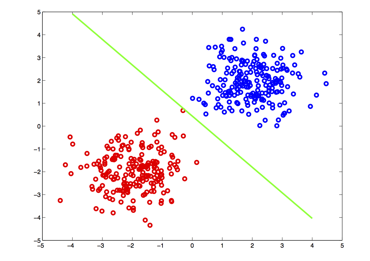
Algorithms that search for such linear boundaries are known as linear learning algorithms: these methods enjoy good statistical properties and are computationally efficient. Unfortunately, data is not typically linearly separable, as seen below.

To classify these points, an algorithm is needed that can compute nonlinear boundaries. One of the most successful such methods is the kernel support vector machine (SVM) [2,3]. A kernel is a real-valued function whose input is a pair of datapoints, typically written as k(x,y), where x and y lie in some domain Ω. Kernels have to be symmetric, i.e. k(x,y) = k(y,x), and positive semidefinite, which means given any set of N data points X = [x₁, …, x_N], the N x N Gram matrix K_ij:=k(x_i, x_j) has nonnegative eigenvalues. The amazing fact is that a function k(x,y) meeting these conditions automatically guarantees the existence of a nonlinear map ψ(x) to a kernel space H, such that

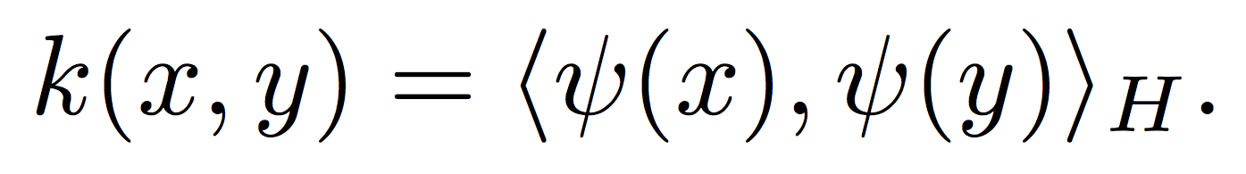
This means that kernel evaluations between points x and y in the input domain are simply inner product evaluations in a high-dimensional kernel space (the Moore-Aronszajn theorem [8]). Researchers have used this fact, and the linearity of the inner product, to devise a large number of nonlinear machine learning algorithms from linear algorithms paired with a kernel function.  Although the most famous such algorithm is the kernel SVM, kernel versions of virtually every linear learning algorithm exist, including perceptrons, linear regression, principal components analysis, k-means clustering, and so on [3]. In each case, the data is mapped to the kernel space, and the linear learning algorithm is applied. The following figures show an example of this basic idea.

The choice of kernel function completely determines the kernel space H. The most popular kernel used in kernel SVMs is the Gaussian kernel function,

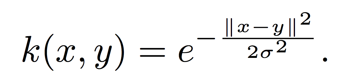
Here, σ is a positive parameter which determines the smoothness of the kernel. The Gaussian kernel actually generates an infinite-dimensional space [4]. Since  kernel spaces can be of such high dimension, a work-around called the ‘kernel trick’ is used to cast the problem into dual form, which allows solutions to be written in terms of kernel expansions on the data and not the kernel space itself. In the following section, we briefly discuss how to recover at least part of the infinite-dimensional kernel space: our discussion is both technical and informal, and can be safely skimmed by the disinterested reader.

Mathematical Origins: Kernel Diagonalization

The kernel space used in kernel methods did not arise in a vacuum: their roots go back to the following integral operator equation:

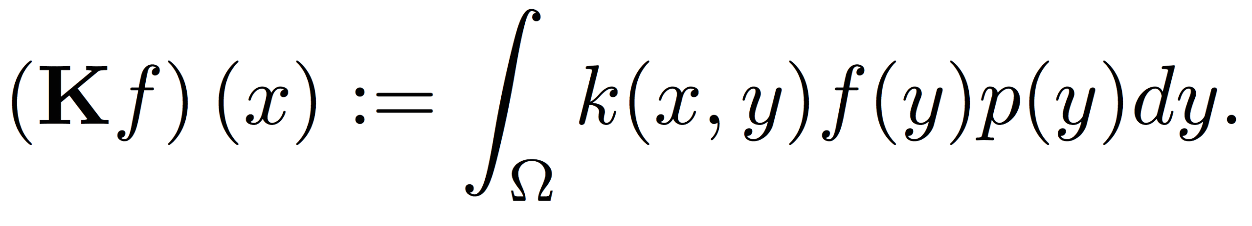
Here, Ω is the domain of the data, p(y) refers to the probability density generating the data, and the operator K maps functions f from the space they reside in to another space generated by the kernel k(x,y).
This equation arose in Ivar Fredholm’s work on mathematical physics in the late 19th century, focusing on partial differential equations with specified boundary conditions. His work inspired other mathematicians, including David Hilbert, who used Fredholm’s insights to create the theory of Hilbert spaces, which were used to great effect in fields such as quantum mechanics and harmonic analysis (signal processing) [5]. The kernel spaces associated with positive-definite kernels are special kinds of Hilbert spaces called reproducing kernel Hilbert spaces (RKHSs): work by mathematicians such as James Mercer and Nachman Aronszajn was instrumental in setting the foundations of this subject [8, 9]. Their work was utilized in turn by statisticians and probabilists working on Gaussian processes [10], and applied mathematicians working on function interpolators such as splines and kriging [11, 12]. After Cortes’ and Vapnik’s seminal paper on support vector machines [2], the theory of RKHSs became firmly embedded in the machine learning landscape.

Returning to the equation at hand, the first thing to note is that linear operators such as K are simply continuous versions of matrices: in fact, if the probability density consists of a set of N samples, it can be shown that the all of the information associated to the integral operator equation above is encoded in the N x N Gram matrix computed from all pairs of the data. Secondly, since the kernel is symmetric, the operator (matrix) can be diagonalized into a set of eigenvalues and eigenfunctions as

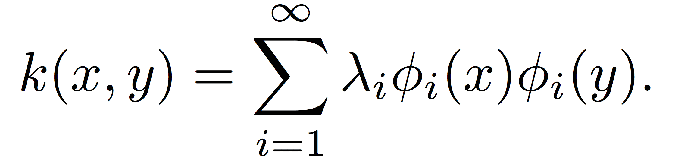
Here, the λ’s denote the eigenvalues, and the Φ’s represent the eigenfunctions: the latter form a basis for the RKHS the kernel creates, with the largest eigenvalues corresponding to the most dominant directions. Using the above equation and the inner product equation in the first section, we can recover the nonlinear kernel map as

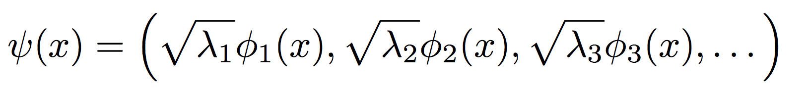
In summary, kernels can be diagonalized and used to construct a kernel map with the most dominant directions: this allows us a direct peek at a projection of the data in the space it resides in!

Using Kernel Eigenfunctions to Visualize Model Data

As mentioned earlier, at Pindrop, most of our models utilize Gaussian kernel SVMs. I now show an example of data from a Phoneprint™ model embedded in the RKHS. A Phoneprint™ is a classification model that distinguishes data from one particular fraudster versus other customers. In this particular example, the total number of samples was about 8000 vectors, with the classes evenly balanced, in a 145-dimensional space. The visualization process consists of the following steps:

1. Perform a grid search over the parameters of the Gaussian kernel, and use the classification accuracy of the SVM to select the correct parameters for the kernel.
2. Use the chosen parameter σ to construct an 8000 x 8000 Gram matrix from the data.
3. Compute the eigenvectors and eigenvalues of the Gram matrix.
4. Use the eigenvectors and eigenvalues to compute the top k eigenfunctions of the integral operator (see [6] to see how this is done in detail).
5. Compute the final feature map as defined in the previous section.
6. Map the dataset X into k-dimensional space using feature map.

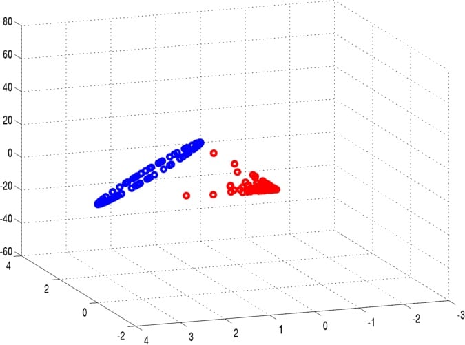
Due to the eigendecomposition step, this process has a computational of O(N³). The end result of mapping the Phoneprint™ data with k=3 is shown below.

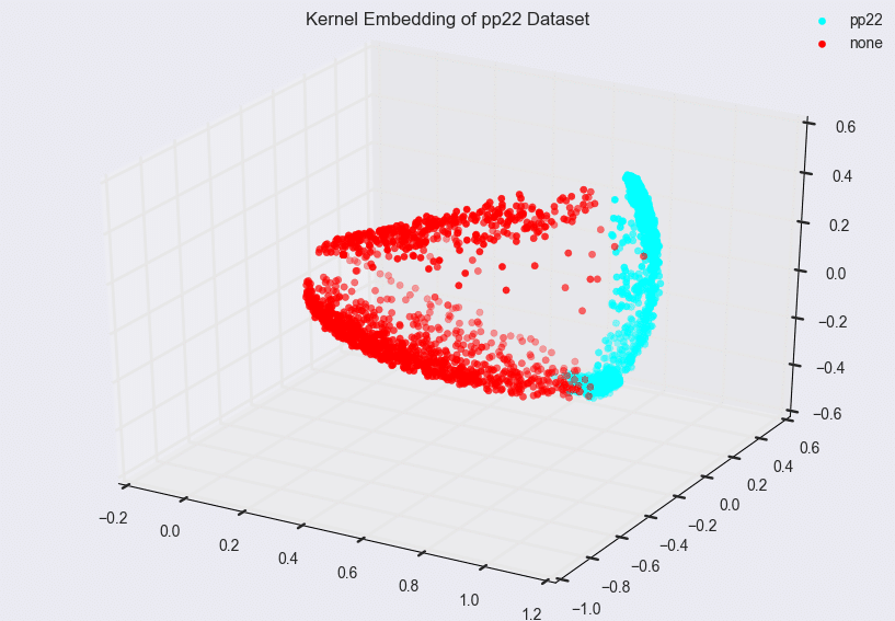
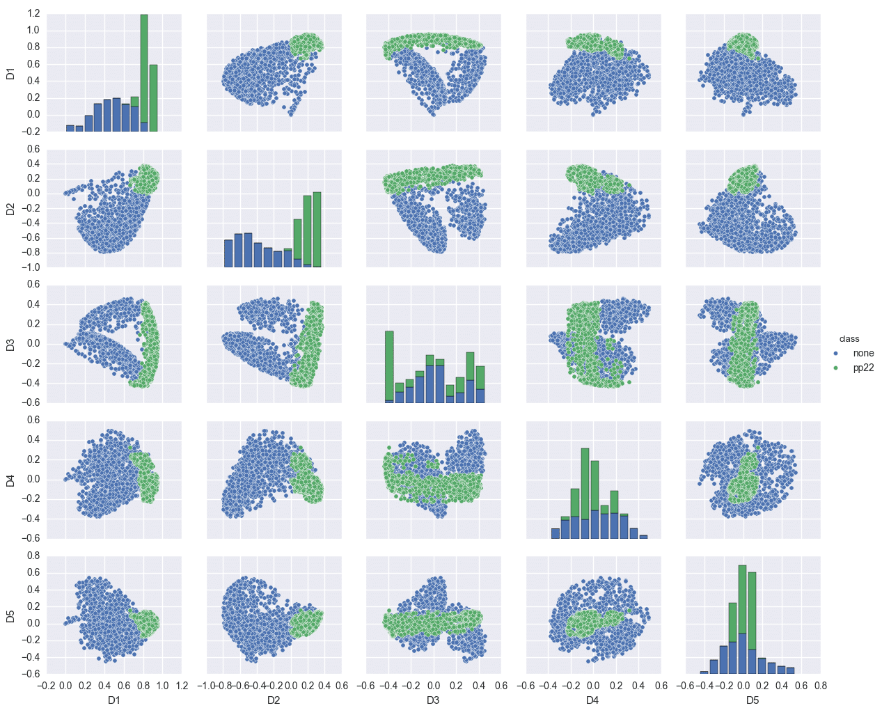
This Phoneprint™ model shows the surprising fact that even though the kernel space is infinite-dimensional, fraudsters can be distinguished almost perfectly from regular customers using very few dominant eigenfunctions!

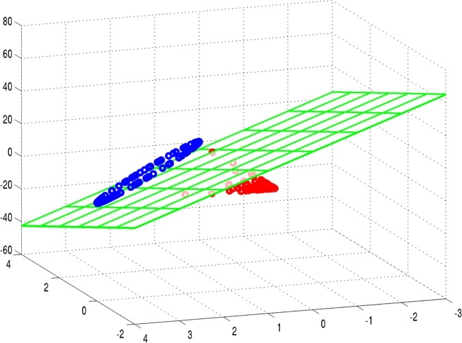
Such pictures can also be used to identify problematic areas in modeling. Consider the following model trained again on 8000 vectors, with the classes evenly balanced, in a 145-dimensional space, but where the data was obtained from some other source.

 

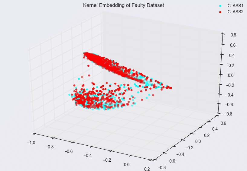
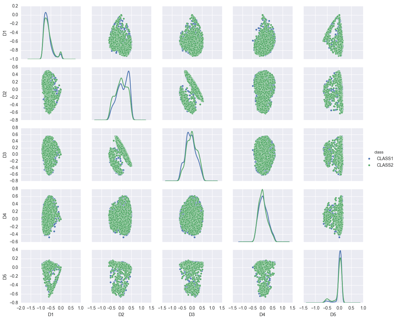
In this example, the first few eigenfunctions do not suffice for model separation. In fact, the classification accuracy of this model is much lower than the Phoneprint™ model, which usually indicates that either the feature space induced by the kernel is not a good choice, or that the vector space the input data is mapped to is not a good choice. Typically, it’s a combination of both: in the feature extraction step, the right features can make or break the learning problem. Similarly, if the kernel space chosen does not allow for a good representation of the feature data (compare the Phoneprint™ model to the faulty data model here), finding a good classifier becomes difficult, if not outright impossible. Finally, the nonlinear maps associated with kernels are not the only choice available: other strategies allow for the construction of completely different classes of nonlinear maps. An example of this that has gained considerable notoriety is deep learning, which uses stacked autoencoders or restricted Boltzman machines to learn extremely sophisticated nonlinear maps from the data [7]. Future work at Pindrop will explore these options as well!

References

1. Murphy, Kevin P. Machine learning: a probabilistic perspective. MIT Press, 2012.
2. Cortes, Corinna, and Vladimir Vapnik. Support-vector networks. Machine Learning 20.3 (1995): 273-297.
3. Shawe-Taylor, John, and Nello Cristianini. Kernel methods for pattern analysis. Cambridge University Press, 2004.
4. Schölkopf, Bernhard, and Christopher JC Burges. Advances in kernel methods: support vector learning. MIT Press, 1999.
5. O’Connor, John J. & Robertson, Edmund F.. (2015). The MacTutor History of Mathematics archive, https://www-history.mcs.st-andrews.ac.uk/. Retrieved at June 17, 2015
6. Williams, Christopher, and Matthias Seeger. “Using the Nyström method to speed up kernel machines.” Proceedings of the 14th Annual Conference on Neural Information Processing Systems. No. EPFL-CONF-161322. 2001.
7. Bengio, Yoshua. “Learning deep architectures for AI.” Foundations and trends® in Machine Learning 2.1 (2009): 1-127.
8. Aronszajn, Nachman. “Theory of reproducing kernels.” Transactions of the American mathematical society (1950): 337-404.
9. Mercer, James. “Functions of positive and negative type, and their connection with the theory of integral equations.” Philosophical transactions of the royal society of London. Series A, containing papers of a mathematical or physical character (1909): 415-446.
10. Dudley, Richard M. Real analysis and probability. Vol. 74. Cambridge University Press, 2002.
11. Stein, Michael L. Interpolation of spatial data: some theory for kriging. Springer Science & Business Media, 2012.
12. Wahba, Grace. Spline models for observational data. Vol. 59. SIAM, 1990.